Adjacency matrix

In mathematics and computer science, an adjacency matrix is a means of representing which vertices of a graph are adjacent to which other vertices. Another matrix representation for a graph is the incidence matrix.

Specifically, the adjacency matrix of a finite graph G on n vertices is the n × n matrix where the nondiagonal entry a_ij is the number of edges from vertex i to vertex j, and the diagonal entry a_ii, depending on the convention, is either once or twice the number of edges (loops) from vertex i to itself. Undirected graphs often use the former convention of counting loops twice, whereas directed graphs typically use the latter convention. There exists a unique adjacency matrix for each graph (up to permuting rows and columns), and it is not the adjacency matrix of any other graph. In the special case of a finite simple graph, the adjacency matrix is a (0,1)-matrix with zeros on its diagonal. If the graph is undirected, the adjacency matrix is symmetric.

The relationship between a graph and the eigenvalues and eigenvectors of its adjacency matrix is studied in spectral graph theory.

1 Examples
2 Adjacency matrix of a bipartite graph
3 Properties
4 Variations
5 Data structures
6 References
7 External links

Examples

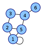
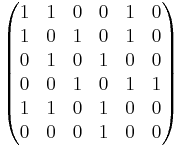
Here is an example of a labeled graph and its adjacency matrix. The convention followed here is that an adjacent edge counts 1 in the matrix for an undirected graph. (X,Y coordinates are 1-6)

Labeled graph	Adjacency matrix
	$\begin{pmatrix} 1 & 1 & 0 & 0 & 1 & 0\\ 1 & 0 & 1 & 0 & 1 & 0\\ 0 & 1 & 0 & 1 & 0 & 0\\ 0 & 0 & 1 & 0 & 1 & 1\\ 1 & 1 & 0 & 1 & 0 & 0\\ 0 & 0 & 0 & 1 & 0 & 0\\ \end{pmatrix}$

The adjacency matrix of a complete graph is all 1's except for 0's on the diagonal.
The adjacency matrix of an empty graph is a zero matrix.

Adjacency matrix of a bipartite graph

The adjacency matrix A of a bipartite graph whose parts have r and s vertices has the form

$A = \begin{pmatrix} O & B \\ B^T & O \end{pmatrix},$

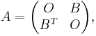
where B is an r × s matrix and O is an all-zero matrix. Clearly, the matrix B uniquely represents the bipartite graphs, and it is commonly called its biadjacency matrix.

Formally, let G = (U, V, E) be a bipartite graph or bigraph with parts 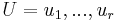$U={u_1,..., u_r}$ and $V={v_1,..., v_s}$ . An r x s 0-1 matrix B is called the biadjacency matrix if $B_{i,j} = 1$ iff $(u_i, v_j) \in E$ .

If G is a bipartite multigraph or weighted graph then the elements $B_{i,j}$ are taken to be the number of edges between or the weight of $(u_i, v_j)$ respectively.

Properties

The adjacency matrix of an undirected simple graph is symmetric, and therefore has a complete set of real eigenvalues and an orthogonal eigenvector basis. The set of eigenvalues of a graph is the spectrum of the graph.

Suppose two directed or undirected graphs $G_1$ and $G_2$ with adjacency matrices $A_1$ and $A_2$ are given. $G_1$ and $G_2$ are isomorphic if and only if there exists a permutation matrix $P$ such that

$P A_1 P^{-1} = A_2.$

In particular, $A_1$ and $A_2$ are similar and therefore have the same minimal polynomial, characteristic polynomial, eigenvalues, determinant and trace. These can therefore serve as isomorphism invariants of graphs. However, two graphs may possess the same set of eigenvalues but not be isomorphic – one cannot 'hear' (reconstruct, or 'inverse-scatter') the shape of a graph.

If A is the adjacency matrix of the directed or undirected graph G, then the matrix Aⁿ (i.e., the matrix product of n copies of A) has an interesting interpretation: the entry in row i and column j gives the number of (directed or undirected) walks of length n from vertex i to vertex j. This implies, for example, that the number of triangles in an undirected graph G is exactly the trace of A³ divided by 6.

The main diagonal of every adjacency matrix corresponding to a graph without loops has all zero entries.

For $\left( d \right)$ -regular graphs, d is also an eigenvalue of A, for the vector $v=\left( 1,...,1 \right)$ , and $G$ is connected if and only if the multiplicity of $d$ is 1. It can be shown that $-d$ is also an eigenvalue of A if G is connected bipartite graph. The above are results of Perron–Frobenius theorem.

Variations

The Seidel adjacency matrix or (0,−1,1)-adjacency matrix of a simple graph has zero on the diagonal and entry $a_{ij} = -1$ if ij is an edge and +1 if it is not. This matrix is used in studying strongly regular graphs and two-graphs.

A distance matrix is like a higher-level adjacency matrix. Instead of only providing information about whether or not two vertices are connected, also tells the distances between them. This assumes the length of every edge is 1. A variation is where the length of an edge is not necessarily 1.

Data structures

When used as a data structure, the main alternative for the adjacency matrix is the adjacency list. Because each entry in the adjacency matrix requires only one bit, they can be represented in a very compact way, occupying only ${n^2} / 8$ bytes of contiguous space, where $n$ is the number of vertices. Besides just avoiding wasted space, this compactness encourages locality of reference.

On the other hand, for a sparse graph, adjacency lists win out, because they do not use any space to represent edges which are not present. Using a naïve array implementation on a 32-bit computer, an adjacency list for an undirected graph requires about $8 e$ bytes of storage, where $e$ is the number of edges.

Noting that a simple graph can have at most $n^2$ edges, allowing loops, we can let $d = e / n^2$ denote the density of the graph. Then, $8 e > n^2 / 8$ , or the adjacency list representation occupies more space, precisely when $d > 1/64$ . Thus a graph must be sparse indeed to justify an adjacency list representation.

Besides the space tradeoff, the different data structures also facilitate different operations. Finding all vertices adjacent to a given vertex in an adjacency list is as simple as reading the list. With an adjacency matrix, an entire row must instead be scanned, which takes O(n) time. Whether there is an edge between two given vertices can be determined at once with an adjacency matrix, while requiring time proportional to the minimum degree of the two vertices with the adjacency list.

References

Thomas H. Cormen, Charles E. Leiserson, Ronald L. Rivest, and Clifford Stein (2001), Introduction to Algorithms, second edition. MIT Press and McGraw-Hill. ISBN 0-262-03293-7. Section 22.1: Representations of graphs, pp. 527–531.

Chris Godsil and Gordon Royle (2001), Algebraic Graph Theory. New York: Springer-Verlag. ISBN 0-387-95241-1

External links

Fluffschack — an educational Java web start game demonstrating the relationship between adjacency matrices and graphs.